Relaxation modulus comparison of tank and modified asphalt binder by means of experimental and simple numerical approaches

Ki Hoon Moon

doi:10.22702/jkai.2024.14.2.28

Preview

Scientific Paper

Journal of the Korean Asphalt Institute. 31 December 2024. 306-313
https://doi.org/10.22702/jkai.2024.14.2.28

Relaxation modulus comparison of tank and modified asphalt binder by means of experimental and simple numerical approaches

Ki Hoon Moon¹^*

¹Principal Researcher, Korea Expressway Corporation Research Division

^{*Corresponding Author}

License (open-access, https://creativecommons.org/licenses/by-nc/4.0/):

This is an Open-Access article distributed under the terms of the Creative Commons Attribution Non-Commercial License (https://creativecommons.org/licenses/by-nc/4.0) which permits unrestricted non-commercial use, distribution, and reproduction in any medium, provided the original work is properly cited.

ABSTRACT

For bituminous material such as asphalt pavement material, low temperature cracking is one of significant distresses. During the cold session, several macro cracks can be occurred due to too brittle characteristic of asphalt material. To evaluate the level of brittleness of given asphalt binder, low temperature creep test is widely used. In this low temperature creep test of asphalt material, creep stiffness is computed and this value can be converted into relaxation modulus: one of significant criteria for evaluating low temperature performance of asphalt binder, with various mathematical approaches. In this paper, relaxation modulus of modified asphalt binder with two different mathematical approaches, was computed, analyzed then compared. It was found that the two different computation methods can successfully provide upper and lower bounds of relaxation modulus of given asphalt binder.

Keywords

Low temperature cracking

Creep stiffness

Relaxation modulus

Mathematical approach

MAIN

1. Introduction
2. Information on experimental work (BBR creep test)
3. Relaxation modulus: E(t), conversion approaches
3.1 Simple power law function approach
3.2 Hopkins and Hamming’s algorithm (1967)
4. Data analysis
5. Summary and conclusions

1. Introduction

Thermal cracking is a crucial distress for asphalt pavements especially in northern U.S. and Canada (Moon, 2010; Moon et al., 2013). When temperature drops below 0°C, thermal stress originated and increase in the restricted asphalt layers. When the temperature drops below a limit value known as critical temperature, finally low temperature cracking occurs (Moon, 2010; Moon et al., 2013). Low temperature cracking is source of significant negative effects on asphalt pavement performance; due development of surface cracks (i.e. including micro and macro cracks) water infiltration in pavement structure occurs. Finally, this leads significant pavement deteriorations (e.g. low temperature cracking, large pavement deformation etc.) which provide crucially negative effects to its users (Marasteanu et al., 2009; Moon, 2010).

Due to this reason, many road agencies are trying considerable efforts to maintain asphalt pavement performances and network systems at acceptable levels (Cannone Falchetto et al., 2014). Various experimental approaches have been introduced during the past decades to characterize the low temperature behavior (e.g. viscoelastic characteristics) of bituminous materials (Marasteanu et al., 2009; Moon, 2010; Moon et al., 2014; Cannone Falchetto et al., 2014). One good example is the low temperature creep test (Marasteanu et al., 2009; Moon, 2010; AASHTO T313-12, 2012). On this experimental test, creep stiffness: S(t), creep compliance: J(t) can be easily computed based on current specification (AASHTO T313-12, 2012). Then an important material performance criterion, relaxation modulus: E(t), can be calculated by means of different mathematical approaches (Moon, 2010; Moon et al., 2013; Cannone Falchetto et al., 2014). However, not many studies have considered the numerical comparisons of E(t) results.

In this paper, two different mathematical approaches (e.g. power law transfer function and Hopkins & Hamming’s algorithm) were considered to convert J(t) to E(t). As an experimental work, Bending Beam Rheometer (BBR) low temperature creep test was considered (AASHTO M320-10, 2010; AASHTO T313-12, 2012). Then the relaxation modulus: E(t), results were analyzed and compared visually to derive engineering meanings.

2. Information on experimental work (BBR creep test)

Two different asphalt binders were prepared in this paper (e.g. one is original tank binder and the other one is modified binder). More detailed information on the prepared materials is shown in Table 1.

Table 1.

Prepared asphalt binders

ID	Binder Description	Material Source	PG	Aging Condition
A	Asphalt binder Plain	University of Minnesota (U.S.)	58-28	Long term (PAV) Test temp: -18ºC
B	Asphalt binder SBS modified	University of Minnesota (U.S.)	64-34	Long term (PAV) Test temp: -24ºC

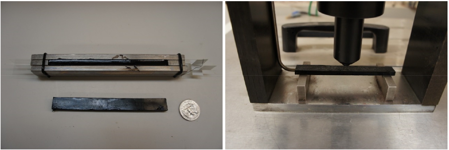
In BBR creep test (AASHTO T313-12, 2012, see Fig. 1), low temperature creep stiffness: S(t), can be computed as follows:

1) BBR creep tests were performed on thin asphalt binder beams (102.0 ± 5 mm × 12.7 ± 0.5 mm × 6.25 ± 0.5 mm) according to the current AASHTO specification (AASHTO T313-12, 2012).

2) In BBR creep test, the mid-span deflection, $δ$ (t), of an asphalt binder specimen is measured for the entire duration of the test (total = 240 s), then the creep stiffness, S(t) and the m-value (slope of logarithmic S(t) vs time curve) can be computed as:

(1)

S (t) = \frac{σ}{ε (t)} = \frac{P ∙ l^{3}}{4 ∙ b ∙ h^{3} ∙ δ (t)} = \frac{1}{D (t)}

(2)

m (t) = | \frac{d \log S (t)}{d \log t} |

3) In Equations (1) and (2), S(t) is the flexural creep stiffness; D(t) is the creep compliance; σ is the maximum bending stress in the beam; ε(t) is the bending strain; P is the constant applied load (980 ± 50 mN); l is the length of specimen (102 ± 5 mm); b is the width of specimen (12.7 ± 0.5 mm); h is height of specimen (6.25 ± 0.5 mm); $δ$ (t) is the deflection at the mid-span of the beam, and t is testing time (0~240 s).

4) Then, relaxation modulus: E(t), was computed based on computed S(t) (and/or D(t)) and compared visually. It needs to be mentioned that computation of E(t) is crucial because results of E(t) can be moved on to thermal stress calculation: one of significant low temperature properties of asphalt material especially at low temperature condition.

https://cdn.apub.kr/journalsite/sites/jkai/2024-014-02/N0850140220/images/jkai_2024_142_306_F1.jpg

Fig. 1.

BBR asphalt binder specimen (left) and BBR testing equipment setup (right)

3. Relaxation modulus: E(t), conversion approaches

Conventionally, J(t) and E(t) can be inter-related by means of the convolution integral as (Findley et al., 1976; Ferry, 1980; Moon, 2010; Moon et al., 2013):

(3)

\int_{0}^{t} E (t - τ) ∙ J (τ) d τ = t

(4)

\int_{0}^{t} E (τ) ∙ J (t - τ) d τ = t

where t > 0

Through Laplace transformation application, Equations (3) or (4) can be re-expressed as:

(5)

E (s) ∙ J (s) = \frac{1}{s^{2}}

where s > 0 is the Laplace transformation parameter.

However, in many cases the expressions for E(t) and J(t) cannot be easily computed in the Laplace domain. Therefore, various numerical approaches are considered as an alternative and convenient method for solving the convolution integral in Equations (3) and (4).

3.1 Simple power law function approach

In previous researches, it was found that values of J(t) and E(t) can be interrelated through a simple power-law functions as follows (Ebrahimi et al., 2014):

(6)

E (t) = E_{1} ∙ t^{n}

(7)

J (t) = J_{1} ∙ t^{- n}

where E₁, J₁ and n are positive constants. With applications of Laplace transformation approach and Euler reflective formula, E(t) and J(t) can be inter-related as (see Equations (8) and (9)):

(8)

E (t) ∙ D (t) = \frac{\sin (n ∙ π)}{n ∙ π}

where parameter n can be expressed as:

(9)

n = | \frac{d \log D (t)}{\log τ} |_{τ = t} o r n = | \frac{d \log E (t)}{\log τ} |_{τ = t}

These power-law approximation methods provide very good results when D(t), and/or J(t), is close to a straight line in a log-log scale plot against time.

3.2 Hopkins and Hamming’s algorithm (1967)

In this paper, a simple numerical algorithm introduced by Hopkins and Hamming (1967) is applied to compute E(t) from J(t). The main computational steps for obtaining E(t) can be summarized:

1) Select a time interval as:

(10)

t_{0} = 0, t_{1} = 1, t_{2} = 2, . . . t_{n} = n

2) Express the integral form of J(t) as:

(11)

f (t) = \int_{0}^{t} J (t) d t

3) From Equation (11), f(t) can be re-expressed by means of trapezoid integration rule:

(12)

f (t_{n + 1}) = f (t_{n}) + \frac{1}{2} ∙ (J (t_{n + 1})) + J (t_{n})) ∙ (t_{n + 1} - t_{n})

4) Equations (10) to (12) can be modified using the above Equation (12) as:

(13)

t_{n + 1} = \int_{0}^{t_{n} + 1} E (τ) ∙ J (t_{n + 1} - τ) d τ = \sum_{i = 0}^{n} \int_{t_{i}}^{t_{i} + 1} E (τ) ∙ J (t_{n + 1} - τ) d τ

5) From Equation (13), each integral element can be approximated as:

(14)

\int_{t_{i}}^{t_{i} + 1} E (τ) ∙ J (t_{n + 1} - τ) d τ = - E (t_{i + 1 / 2}) ∙ [f (t_{n + 1} - t_{n + 1}) - f (t_{n + 1} - t_{i})]

(15)

Where, t_{i + \frac{1}{2}} = \frac{1}{2} ∙ (t_{i + 1} + t_{i})

6) Equation (14) can be written as:

(16)

t_{n + 1} = - \sum_{i = 0}^{n - 1} E (t_{i + 1 / 2}) ∙ [f (t_{n + 1} - t_{i + 1}) - f (t_{n + 1} - t_{i})] + E (t_{n + 1 / 2}) ∙ f (t_{n + 1} - t_{n})

7) Solving for $E (t_{n + 1 / 2})$ , Equation (16) is:

(17)

E (t_{n + 1 / 2}) = \frac{t_{n + 1} - \sum_{i = 0}^{n - 1} E (t_{i + 1 / 2}) ∙ [f (t_{n + 1} - t_{i}) - f (t_{n + 1} - t_{i + 1})]}{f (t_{n + 1} - t_{n})} = \frac{t_{n + 1} - \sum_{i = 0}^{n - 1} E (t_{i + 1 / 2}) ∙ [f (t_{i + 1}) - f (t_{i})]}{f (t_{n + 1}) - f (t_{n})}

where, $f (t_{0}) = 0, E (t_{0}) = 0, E (t_{1}) = t_{1} / f (t_{1})$

It should be mentioned that Simple Power law method is easy to compute E(t) results however, less on detailed answer. The Hopkins and Hamming’s algorithm can provide more reliable E(t) results but the computation process is a little but complicated.

4. Data analysis

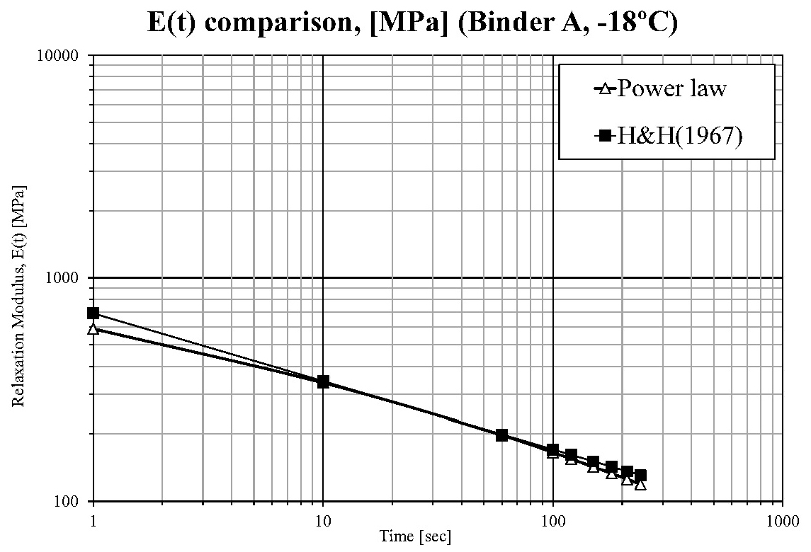
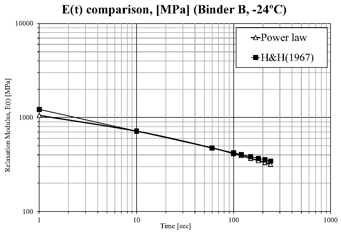
Based on the above theories (i.e. See Section 3), the computed results of E(t) can be presented as follows (i.e. see Figs. 2 and 3).

From the results in Figs. 2 to 3, it was found that the different mathematical approaches can successfully provide upper and lower bounds on E(t) computation working process. This crucial finding can be related to thermal stress computation step and this will be considered as the next research topic.

https://cdn.apub.kr/journalsite/sites/jkai/2024-014-02/N0850140220/images/jkai_2024_142_306_F2.jpg

Fig. 2.

E(t) comparison, binder A (-18°C)

https://cdn.apub.kr/journalsite/sites/jkai/2024-014-02/N0850140220/images/jkai_2024_142_306_F3.jpg

Fig. 3.

E(t) comparison, binder B (-24°C)

5. Summary and conclusions

In this paper, different mathematical approaches for relaxation modulus computation on asphalt material were considered. A simple power law function and Hopkins and Hamming’s algorithm was considered. Finally, it was found that successfully upper and lower bounds on relaxation modulus computation was derived. This means reliable range on low temperature performance computation of asphalt material is available by means of different mathematical approaches. More extensive experimental works and further numerical analysis efforts are needed as future research in this paper.

References

AASHTO M320-10 (2010). Standard Specification for Performance-Graded Asphalt Binder. American Association of State Highway and Transportation Officials (AASHTO).

AASHTO T313-12 (2012). Determining the Flexural Creep Stiffness of Asphalt Binder Using the Bending Beam Rheometer (BBR). American Association of State Highway and Transportation Officials (AASHTO).

Cannone Falchetto, A., Marasteanu, M.O., Balmurugan, S. and Negulescu, I.I. (2014). "Investigation of Asphalt Mixture Strength at Low Temperatures with the Bending Beam Rheometer", Road Materials and Pavement Design, 15(1), pp. 28-44.

10.1080/14680629.2014.926618

Ebrahimi, M.G., Saleh, M. and Gonzalez M.A.M. (2014). "Interconversion between Viscoelastic Functions Using the Tikhonov Regularisation Method and its Comparison with Approximate Techniques", Road Material and Pavement Design, 15(4), pp. 820-840.

10.1080/14680629.2014.924428

Ferry, J.D. (1980). Viscoelastic properties of polymers, 3rd ed., Wiley, New York.

Findley, W.N., Lai, J.S. and Onaran K. (1976). Creep and Relaxation of Nonlinear Viscoelastic Materials. Dover Publications, New York, US.

Hopkins, I.L. and Hamming, R.W. (1967). "On Creep and Relaxation", Journal of Applied Physics, 28(8), pp. 906-909.

10.1063/1.1722885

Marasteanu, M.O., Velasquez, R.A., Cannone Falchetto, A. and Zofka, A. (2009). Development of a Simple Test to Determine the Low Temperature Creep Compliance of Asphalt Mixtures. IDEA Program Final Report, NCHRP-133.

Moon, K.H. (2010). Comparison of thermal stresses calculated from asphalt binder and asphalt mixture creep compliance data, M.S. dissertation, University of Minnesota.

Moon, K.H., Cannone Falchetto, A., and Yeom, W.S. (2014). "Low-Temperature Performance of Asphalt Mixtures Under Static and Oscillatory Loading", Arabian Journal for Science and Engineering, 39(11), pp. 7577-7590.

10.1007/s13369-014-1321-2

Moon, K.H., Marasteanu M.O. and Turos, M. (2013). "Comparison of Thermal Stresses Calculated from Asphalt Binder and Asphalt Mixture Creep Tests", Journal of Materials in Civil Engineering, 25(8), pp. 1059-1067.

10.1061/(ASCE)MT.1943-5533.0000651

Journal of the Korean Asphalt Institute ISSN:2234-0785(Print) 2635-9553(Online) 한국아스팔트학회지

Preview

Relaxation modulus comparison of tank and modified asphalt binder by means of experimental and simple numerical approaches

ABSTRACT

MAIN

Table 1.

Prepared asphalt binders

(1)

(2)

Fig. 1.

BBR asphalt binder specimen (left) and BBR testing equipment setup (right)

(3)

(4)

(5)

(6)

(7)

(8)

(9)

(10)

(11)

(12)

(13)

(14)

(15)

(16)

(17)

Fig. 2.

E(t) comparison, binder A (-18°C)

Fig. 3.

E(t) comparison, binder B (-24°C)

References