

1. Introduction
2. Experimental work
3. Different computation approaches for computing relaxation modulus: E(t)
3.1 Inter-conversion based on Hopkins and Hamming’s algorithm (1967)
3.2 Two approximated inter-conversion approaches for computing E(t)
4. Data analysis
5. Summary and conclusion
1. Introduction
Low temperature cracking so called thermal cracking is one of serious distresses on asphalt pavement especially in Northern U.S. and Canada (Marasteanu et al., 2009; Moon, 2010; Moon et al., 2013; Moon et al., 2014). When temperature drops below 0ºC, thermal stress starts to be increased in restricted asphalt pavement layer. Then crack starts to be initiated when the internal temperature in asphalt layer exceeds the original endurable temperature limit so called critical cracking temperature: TCR. This low temperature cracking provides seriously negative effect on asphalt layer due to infiltration of water and moisture which probably leads to rapid deterioration of pavement layer. Because of this reason many pavement agencies in U.S. and Canada recognize thermal stress as one of the significant pavement performance evaluation parameters (Moon, 2010; Cannone Falchetto et al., 2014).
It is well known that low temperature creep test is required to compute amount of thermal stress on asphalt pavement material numerically (Marasteanu et al., 2009; Moon, 2010; Moon et al., 2014). In creep test, thermal stress can be calculated based on following three steps:
1) Creep compliance: D(t), is computed based on experimental results
2) Then Relaxation modulus: E(t), is computed through various inter-conversion approach
3) By solving one dimensional hereditary integral, thermal stress can be computed.
Therefore, it can be said that computation (and/or estimation) of E(t) is essential for computing thermal stress of given asphalt material. However, the inter-conversion process such as applying numerical analysis approach: Hopkins and Hamming’s algorithm (1967) is relatively complicated therefore not many universities or pavement agencies can compute E(t) from experimental D(t).
In this paper, two simple E(t) computation approaches based on approximated method are introduced. Bending Beam Rheometer (BBR) binder creep test (AASHTO T313-12, 2012) was performed as an experimental work. First, creep stiffness: S(t), and corresponding creep compliance: D(t), was computed based on Euler-Bernoulli beam theory (Moon, 2010). Then relaxation modulus: E(t), was computed based on three methods: two simple approximated methods (will be mentioned later section in this paper) and conventional Hopkins and Hamming’s algorithm (1967). Finally, all the computed results were compared visually. At the end of this paper, the findings, conclusions and recommendations on computing E(t) with different mathematical approaches are mentioned and considered.
2. Experimental work
Two different asphalt binders for conventional Hot Mix Asphalt (HMA) pavement construction were considered in this paper. It needs to be mentioned that only 2 different binders were able to be prepared due to limitations for material supply. The previously known Performance Grade (PG) values of prepared asphalt binder were PG 64-34 and PG 64-28, respectively (AASHTO M 320-10-UL, 2010). Both the binders were prepared from Korea Expressway Corporation Pavement Research Division (KECPRD).
BBR binder test (AASHTO T313-12, 2012) currently mentioned in AASHTO specification was performed as an experimental work. Moreover, all the binders were long-term aged before testing according to the Pressurized Aging Vessel (PAV) (AASHTO R028-12, 2012) procedure. Brief information of prepared material in this paper is shown in Table 1.
Table 1. Information of Prepared Asphalt Binders in This Study
As can be seen in Fig. 1, BBR binder creep test was performed on this asphalt binder beam (102.05 mm 12.70.5 mm 6.250.5 mm) based on the current AASHTO specification (AASHTO T 313-12, 2012). In BBR binder test, the mid-span deflection, δ(t),is measured for 240 seconds with application of constant load amounted 98050 mN.
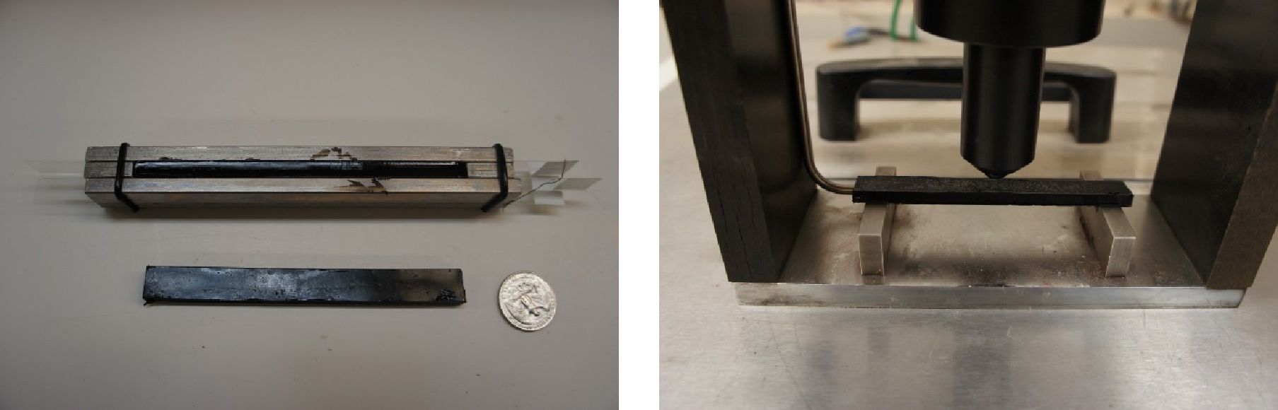
In BBR binder creep test, the creep stiffness: S(t), can easily be computed based on Euler-Bernoulli theory (Moon, 2010) as:
| $$S(t)=\frac1{D(t)}=\frac\sigma{\varepsilon(t)}=\frac{P\cdot l^3}{4\cdot b\cdot h^3\cdot\delta(t)}$$ | (1) |
In Equation (1), S(t) is the flexural creep stiffness; D(t) is the creep compliance; σ is the maximum bending stress in the beam;ε(t) is the bending strain; P is the constant applied load (98050 mN); l is the length of specimen (1025 mm); b is the width of specimen (12.70.5 mm); h is height of specimen (6.250.5 mm); δ(t) is the deflection at the mid-span of the beam, and t is testing time (0~240 s).
3. Different computation approaches for computing relaxation modulus: E(t)
3.1 Inter-conversion based on Hopkins and Hamming’s algorithm (1967)
It is well known that the creep compliance, D(t), and the relaxation modulus, E(t) of a viscoelastic material are inter-correlated by the convolution integral as (Findley et al., 1976; Ferry, 1980):
| $$\int_0^tE(t-\tau)\cdot D(\tau)d\tau=t$$ | (2) |
| $$\int_0^tE(\tau)\cdot D(t-\tau)d\tau=t$$ | (3) |
Where t > 0
It needs to be mentioned that solving Equations (2) or (3) is relatively complex in most cases. Therefore, not an analogical approach but a numerical computation approach (and/or algorithm) is needed to solve the convolution integral (e.g. Equations (2) and (3)). Hopkins and Hamming’s algorithm (1967) is widely used for computing E(t) from experimental D(t) (see Equation (1)). The following steps are need for computing E(t) by means of Hopkins and Hamming’s algorithm (1967):
| $$\mathrm{Select}\;\mathrm a\;\mathrm{time}\;\mathrm{interval}\;\mathrm{as}:\;t_0=0,\;t_1=1,\;t_2=2,\cdots t_n=n$$ | (4) |
| $${\mathrm a.\;\mathrm{Express}\;D(t)\;\mathrm{as}}:\;f(t)=\int_0^tD(t)dt$$ | (5) |
b. From Equation (5), can be calculated with the trapezoid integration rule as:
| $$f(t_{n+1})=f(t_n)+\frac12\cdot(D(t_{n+1})+D(t_n))\cdot(t_{n+1}-t_n)$$ | (6) |
c. Equations (2)~(3) can be modified by using Equation (6) as:
| $$t_{n+1}=\int_0^{t_n+1}E(\tau)\cdot D(t_{n+1}-\tau)d\tau=\sum_{i=0}^n\int_{t_i}^{t_i+1}E(\tau)\cdot D(t_{n+1}-\tau)d\tau$$ | (7) |
d. From Equation (7), each element of the integral can be approximated as:
| $$\int_{t_i}^{t_i+1}E(\tau)\cdot D(t_{n+1}-\tau)d\tau=-E(t_{i+1/2})\cdot\lbrack f(t_{n+1}-t_{n-1})-f(t_{n+1}-t_i)\rbrack$$ | (8) |
| $$\mathrm{Where},\;t_{i+\frac12}=\frac12\cdot(t_{i+1}+t_i)$$ | (9) |
e. Equation (8) can be then re-expressed as:
| $$t_{n+1}=-\sum_{i=0}^{n-1}E(t_{i+1/2})\cdot\lbrack f(t_{n+1}-t_{i+1})-f(t_{n+1}-t_i)\rbrack+E(t_{n+1/2})\cdot f(t_{n+1}-t_n)$$ | (10) |
f. Solving for , Equation (10) can be expressed as:
where,
Based on the above computation procedure (e.g. Equations (2) to (11)), relaxation modulus: E(t) can finally computed from experimental creep compliance: D(t), numerically.
3.2 Two approximated inter-conversion approaches for computing E(t)
Based on the convolution integral mentioned above (i.e. Equations (2) and (3)) and Equation (12) an approximated relationship between D(t) and E(t) was introduced by Denby (1975) as:
| $$\begin{array}{l}\mathbf L\left[\int_0^tE(\tau)\cdot D(t-\tau)d\tau\right]=\mathbf L\lbrack t\rbrack\\\Rightarrow\overline E(s)\cdot\overline D(s)=\frac1{s^2}\end{array}$$ | (12) |
| $$E(t)\cdot D(t)=\frac1{1+{\displaystyle\frac{n^2\cdot\pi^2}6}}$$ | (13) |
In Equation (13), parameter n means
| $$n={\left|\frac{d\log D(t)}{\log\tau}\right|}_{\tau=t}\;\mathrm{or}\;n={\left|\frac{d\log E(t)}{\log\tau}\right|}_{\tau=t}$$ | (14) |
Christensen (1982) also introduced an approximated relationship between D(t) and E(t) based on real and imaginary parts of the complex modulus function as:
| $$E(t)\cdot D(t)=\frac1{1+{\displaystyle\frac{n^2\cdot\pi^2}4}}$$ | (15) |
In Equation (15), parameter n means same as mentioned in Equation (14).
4. Data analysis
After the BBR binder creep experimental work, three different inter-conversion models previously mentioned above were set as follows then compared:
1. Model 1: Hopkins and Hamming’s algorithm (1967) (Equation (11))
2. Model 2: Christensen’s (1982) approximated relationship (Equation (14))
3. Model 3: Denby’s (1975) approximated relationship (Equation (12))
The computed results of creep stiffness: S(t), and Relaxation modulus: E(t), are shown in Figs. 2 to 3 and Tables 2 and 3, respectively.
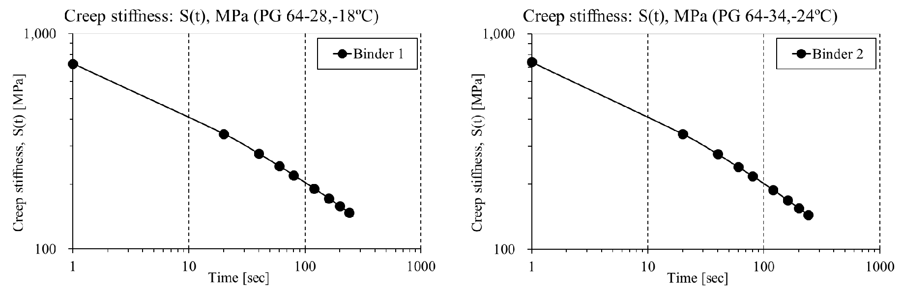
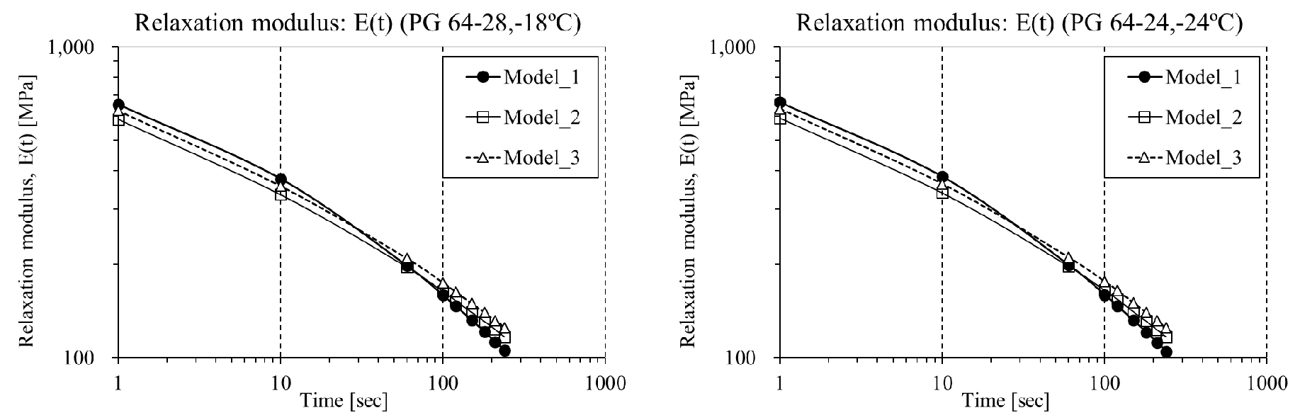
Table 2. Computed Results of Relaxation Modulus: E(t)
Asphalt Binder 1 (PG 64-28) Tested at –18°C
| Time (sec) | Relaxation modulus: E(t), by different Inter conversion model (Model 1~3) | ||
|
Model 1 Hopkins and Hamming’s algorithm (1967) |
Model 2 Christensen (1982) |
Model 3 Denby (1975) | |
| 1 | 653 | 585 | 624 |
| 10 | 375 | 342 | 357 |
| 60 | 196 | 194 | 209 |
| 100 | 158 | 162 | 174 |
| 120 | 145 | 152 | 163 |
| 150 | 132 | 140 | 149 |
| 180 | 121 | 131 | 138 |
| 210 | 112 | 123 | 130 |
| 240 | 104 | 114 | 125 |
Table 3. Computed Results of Relaxation Modulus: E(t)
Asphalt Binder 2 (PG 64-34) Tested at –24°C
| Time (sec) | Relaxation modulus: E(t), by different Inter conversion model (Model 1~3) | ||
|
Model 1 Hopkins and Hamming’s algorithm (1967) |
Model 2 Christensen (1982) |
Model 3 Denby (1975) | |
| 1 | 665 | 592 | 632 |
| 10 | 383 | 339 | 362 |
| 60 | 199 | 197 | 210 |
| 100 | 159 | 164 | 176 |
| 120 | 146 | 154 | 164 |
| 150 | 131 | 140 | 150 |
| 180 | 120 | 131 | 140 |
| 210 | 112 | 123 | 131 |
| 240 | 104 | 117 | 125 |
From the results in Fig. 3 and Tables 2 to 3, some crucial findings could be derived. First, the highest values of E(t) were predicted at initial testing time then the lowest E(t) predictions were generated after 100 testing seconds in case of applying conventional Hopkins and Hamming’s algorithm (1967) compared to the other two computation approaches (i.e. Christensen (1982) and Denby (1975) approximation). In other words, it can be said that more flexible E(t) estimation trends are derived in case of using conventional Hopkins and Hamming’s algorithm (1967) comparted to the other two approximated approaches. In case of two approximated approaches comparison, Model 3 (i.e. Denby’s (1975) approximation) presented relatively higher values of E(t) predictions compared to use of Model 2 (i.e. Christensen's (1982) approximation) even though similar data generation trends were observed. Based on the findings, it can be said that by using these three different E(t) generation approaches the upper and lower bounds of E(t) values can be predicted successfully. Furthermore, these results may provide successful upper and lower bounds on thermal stress and corresponding critical cracking temperature computation (Moon, 2010).
5. Summary and conclusion
In this paper, three different computation approaches for estimating relaxation modulus values from the experimental creep compliance data were introduced then visually compared. Conventional however, sophisticated Hopkins and Hamming’s algorithm (1967) and other two approximated methods: Chistensen’s (1982) and Denby’s (1975) approaches were considered. As a result, it was found that by using three different computation approaches upper and lower bounds of relaxation modulus estimation can successfully be derived. Based on the findings providing upper and lower bounds of thermal stress and corresponding critical cracking temperature of asphalt binder can also be available in the further research.
